I remember when I first started on server-side applications – the kind that need to persist data – and not getting what the big deal about databases was. Why are databases such a big thing? Can’t we just store some data on disk and read / write from it when we need to? (Spoiler: no.)
Once I started working with real-life applications instead of just hobby projects, I realised that databases are basically magic, and SQL is the arcane tongue that allows you to channel that magic. In fact, it’s easy to think of databases like a black box where you make sure your tables are indexed sensibly and your queries aren’t doing anything silly, and the rest just happens.
But really, databases aren’t that complicated. I mean, they kind of are but if you dig inside the database engine a bit, you realise that it’s really just some immensely powerful and clever abstractions and that, like most software, most of the actual complexity in these pieces of software comes from the edge cases, often around concurrency.
I’d like crack open the hard shell of database engines with some friendly introductions to those who are familiar with relational databases but don’t know their inner machinations. I’m going to talk about PostgreSQL because that’s what I’m most familiar with, and it’s also the most popular database in use by developers according to the Stack Overflow Developer Survey 2023 and Stack Overflow Developer Survey 2024.
To start things off, I’m going to discuss how Postgres actually stores data on disk. I mean, it’s all just files, right?
Loading a nice fresh Postgres install
Postgres stores all its data in a directory sensibly called /var/lib/postgresql/data 1 . Let’s spin up an empty Postgres installation with Docker and mount the data directory in a local folder so that we can see what’s going on in there. (Feel free to follow along and explore the files for yourself!)
1docker run --rm -v ./pg-data:/var/lib/postgresql/data -e POSTGRES_PASSWORD=password postgres:16You should see a bunch of text saying all kinds of interesting things like selecting dynamic shared memory implementation ... posix and performing post-bootstrap initialization ... ok and then eventually LOG: database system is ready to accept connections. Now kill the server with ctrl-C so that we can have a look at what files have been created.
1$ ls -l pg-data2drwx------ - base/3drwx------ - global/4drwx------ - pg_commit_ts/5drwx------ - pg_dynshmem/6.rw-------@ 5.7k pg_hba.conf7.rw-------@ 2.6k pg_ident.conf8drwx------ - pg_logical/9drwx------ - pg_multixact/10drwx------ - pg_notify/11drwx------ - pg_replslot/12drwx------ - pg_serial/13drwx------ - pg_snapshots/14drwx------ - pg_stat/15drwx------ - pg_stat_tmp/16drwx------ - pg_subtrans/17drwx------ - pg_tblspc/18drwx------ - pg_twophase/19.rw------- 3 PG_VERSION20drwx------ - pg_wal/21drwx------ - pg_xact/22.rw-------@ 88 postgresql.auto.conf23.rw-------@ 30k postgresql.conf24.rw------- 36 postmaster.optsThere’s a lot of folders here, but if you look, most of them are empty.
Before we dig into these, a quick terminology overview:
| Term | Meaning |
|---|---|
| Database cluster | The term ‘cluster’ is a bit overloaded here - we’re using it the same way that the Postgres docs use it, meaning a single instance of a PostgreSQL server which is running multiple databases on the same machine (where each database is created with create database mydbname). |
| Database connection | When a client connects to the Postgres server, it initiates a database connection. When this happens, Postgres creates a sub-process on the server. |
| Database session | Once the connection has been authenticated, the client has established a session, which it can then use to execute SQL. |
| Transaction a.k.a. tx, xact | SQL is executed within the session inside transactions, which are units of work which are executed, committed and succeed or fail as a single unit of work. If a transaction fails, it is rolled back and all the changes made in the transaction are undone. |
| Snapshot | Each transaction sees its own copy of the database, called its snapshot. If you have multiple sessions reading and writing the same data at the same time, they will in general not see the exact same data but will see different snapshots depending on the exact timing of the transactions. It’s possible to synchronise and export snapshots. |
| Schema | A database consists of multiple schemas (or schemata, if you’re being pretentious), each of which is a logical namespace for tables, functions, triggers and every thing that databases store. The default schema is called public and if you don’t specify a schema, it’s the same as manually specifying public. |
| Table | A database consists of multiple tables, each of which represents a single unordered collection of items with a particular number of columns, each of a specific type. |
| Tablespace | A tablespace is a physical separation (as opposed to schemas, which are a logical separation). We’ll see more about tablespaces later. |
| Row | A table consists of multiple unordered rows, each of which is a single collection of data points defining a specific thing. |
| Tuple | A tuple is very similar to a row, but a tuple is immutable. The state of a specific row at a specific time is a tuple, but a tuple is a more general term for a collection of data points. When you return data from a query, you can get tuples. |
Now let’s do a quick overview of what all these top-level files and folders are for. You don’t need to worry about every single one of these – most of them cover more complicated use cases, which is why they’re empty for us – but I still think it’s interesting to know what each files and folder is for.
| Directory | Explanation |
|---|---|
base/ | Contains a subdirectory for each database. Inside each sub-directory are the files with the actual data in them. We’ll dig into this more in a second. |
global/ | Directly contains files for cluster-wide tables like pg_database. |
pg_commit_ts/ | As the name suggests, contains timestamps for transaction commits. We don’t have any commits or transactions yet, so this is empty. |
pg_dynshmem/ | Postgres uses multiple processes (not multiple threads, although there has been discussion around it) so in order to share memory between processes, Postgres has a dynamic shared memory subsystem. This can use shm_open, shmget or mmap on Linux – by default it uses shm_open. The shared memory object files are stored in this folder. |
pg_hba.conf | This is the Host-Based Authentication (HBA) file which allows you to configure access to your cluster based on hostname. For instance, by default this file has host all all 127.0.0.1/32 trust which means “trust anyone connecting to any database without a password if they’re connecting from localhost”. If you’ve ever wondered why you don’t need to put your password in when running psql on the same machine as the server, this is why. |
pg_ident.conf | This is a user name mapping file which isn’t particularly interesting for our purposes. |
pg_logical/ | Contains status data for logical decoding. We don’t have time to talk about how the Write-Ahead Log (WAL) works in full, but in short, Postgres writes changes that it’s going to make to the WAL, then if it crashes it can just re-read and re-run all the operations in the WAL to get back to the expected database state. The process of turning the WAL back into the high-level operations – for the purposes of recovery, replication, or auditing – is called logical decoding and Postgres stores files related to this process in here. |
pg_multixact/ | ”xact” is what the Postgres calls transactions so this contains status data for multitransactions. Multitransactions are a thing that happens when you’ve got multiple sessions who are all trying to do a row-level lock on the same rows. |
pg_notify/ | In Postgres you can listen for changes on a channel and notify listeners of changes. This is useful if you have an application that wants to action something whenever a particular event happens. For instance, if you have an application that wants to know every time a row is added or updated in a particular table so that it can synchronise with an external system. You can set up a trigger which notifies all the listeners whenever this change occurs. Your application can then listen for that notification and update the external data store however it wants to. |
pg_replslot/ | Replication is the mechanism by which databases can synchronise between multiple running server instances. For instance, if you have some really important data that you don’t want to lose, you could set up a couple of replicas so that if your main database dies and you lose all your data, you can recover from one of the replicas. This can be physical replication (literally copying disk files) and logical replication (basically copying the WAL to all the replicas so that the main database can eb reconstructed from the replica’s WAL via logical decoding.) This folder contains data for the various replication slots, which are a way of ensuring WAL entries are kept for particular replicas even when it’s not needed by the main database. |
pg_serial/ | Contains information on committed serialisable transactions. Serialisable transactions are the highest level of strictness for transaction isolation, which you can read more about in the docs. |
pg_snapshots/ | Contains exported snapshots, used e.g. by pg_dump which can dump a database in parallel. |
pg_stat/ | Postgres calculates statistics for the various tables which it uses to inform sensible query plans and plan executions. For instance, if the query planner knows it needs to do a sequential scan across a table, it can look at approximately how many rows are in that table to determine how much memory should be allocated. This folder contains permanent statistics files calculated form the tables. Understanding statistics is really important to analysing and fixing poor query performance. |
pg_stat_tmp/ | Similar to pg_stat/ apart from this folder contains temporary files relating to the statistics that Postgres keeps, not the permanent files. |
pg_subtrans/ | Subtransactions are another kind of transaction, like multitransactions. They’re a way to split a single transaction into multiple smaller subtransactions, and this folder contains status data for them. |
pg_tblspc/ | Contains symbolic references to the different tablespaces. A tablespace is a physical location which can be used to store some of the database objects, as configured by the DB administrator. For instance, if you have a really frequently used index, you could use a tablespace to put that index on a super speedy expensive solid state drive while the rest of the table sits on a cheaper, slower disk. |
pg_twophase/ | It’s possible to “prepare” transactions, which means that the transaction is dissociated from the current session and is stored on disk. This is useful for two-phase commits, where you want to commit changes to multiple systems at the same time and ensure that both transactions either fail and rollback or succeed and commit |
PG_VERSION | This one’s easy – it’s got a single number in which is the major version of Postgres we’re in, so in this case we’d expect this to have the number 16 in. |
pg_wal/ | This is where the Write-Ahead Log (WAL) files are stored. |
pg_xact/ | Contains status data for transaction commits, i.e. metadata logs. |
postgresql.auto.conf | This contains server configuration parameters, like postgresql.conf, but is automatically written to by alter system commands, which are SQL commands that you can run to dynamically modify server parameters. |
postgresql.conf | This file contains all the possible server parameters you can configure for a Postgres instance. This goes all the way from autovacuum_naptime to zero_damaged_pages. If you want to understand all the possible Postgres server parameters and what they do in human language, I’d highly recommend checking out postgresqlco.nf |
postmaster.opts | This simple file contains the full CLI command used to invoke Postgres the last time that it was run. |
There’s also a file called postmaster.pid which you only see while the Postgres process is actively running, which contains information about the postmaster process ID, what port its listening on, what time it started, etc. We won’t see that here because we stopped our Postgres server to examine the files.
So that was quite intense – don’t worry if you didn’t fully understand what all those things mean – it’s all super interesting stuff but you don’t need to follow most of that to understand what we’re going to talk about, which is the actual database storage.
Exploring the database folders
Okay, so we mentioned the base/ directory above, which has a subdirectory for each individual database in your cluster. Let’s take a look at what we’ve got here:
1$ ls -l pg-data/base2drwx------ - 1/3drwx------ - 4/4drwx------ - 5/Wait, why are there already 3 folders in here? We haven’t even created any databases yet.
The reason is that when you start up a fresh Postgres server, Postgres will automatically create 3 databases for you. They are:
postgres– when you connect to a server, you need the name of a database to connect to, but you don’t always know what the name is. This is also true of database management tools. While it’s not strictly necessary, you can almost always rely on thepostgresdatabase existing – once you’ve connected to this empty, default database, you can list all the other databases on the server, create new databases, and so on.template0,template1– as the name suggests, these databases are templates used to create future databases.
Why are the subdirectories called numbers instead of names?
Well in Postgres, all the system tables for things like namespaces, roles, tables and functions use an Object IDentifier (OID) to identify them. In this case, 1, 4 and 5 are the OIDs for postgres, template0 and template1.
Let’s play with some data
These in-built tables don’t have anything in them and are generally pretty boring, so let’s create ourselves a new database and put them data in so that we can examine the data files themselves.
First, let’s run and detach the Postgres container so that we can query it.
1docker run -d --rm -v ./pg-data:/var/lib/postgresql/data -e POSTGRES_PASSWORD=password postgres:16We could use anything as our play dataset, but I like geography so let’s make a table with some countries in. Let’s download some country data into our container and load it into a new database.
1curl 'https://raw.githubusercontent.com/lukes/ISO-3166-Countries-with-Regional-Codes/master/all/all.csv' \2 --output ./pg-data/countries.csvWe can use a local tool like psql or TablePlus to examine the database, but we’re going to just exec into the container and use psql from inside the container. This way, we don’t have to worry about mapping ports or mismatching psql and Postgres server versions. (Also, it’s easier for everyone to follow along at home.)
1pg_container_id=$(docker ps --filter expose=5432 --format "{{.ID}}")2docker exec -it $pg_container_id psql -U postgresHere we’re getting the container ID of the running Postgres container by filtering by containers which expose port 5432 as Postgres does and putting that into the docker exec command to give us an interactive psql shell. The -U postgres is because the default Postgres user in the official Docker image is postgres, not root which is the psql default.
If that works, you should see something like:
1psql (16.3 (Debian 16.3-1.pgdg120+1))2Type "help" for help.3
4postgres=#
Now let’s create our new database and load the data in: 2
1create database blogdb;2\c blogdb;3
4create table countries (5  id integer primary key generated always as identity,6  name text not null unique,7  alpha_2 char(2) not null,8  alpha_3 char(3) not null,9  numeric_3 char(3) not null,10  iso_3166_2 text not null,11  region text,12  sub_region text,13  intermediate_region text,14  region_code char(3),15  sub_region_code char(3),16  intermediate_region_code char(3)17);18
19copy countries (20  name,21  alpha_2,22  alpha_3,23  numeric_3,24  iso_3166_2,25  region,26  sub_region,27  intermediate_region,28  region_code,29  sub_region_code,30  intermediate_region_code31)32from '/var/lib/postgresql/data/countries.csv'33with csv header;34
35-- Check that the data got loaded into the table ok.36select * from countries limit 10;37
38-- Should say 249.39select count(*) from countries;
Great, so we’ve got a table with 249 rows and a single index corresponding to our unique constraint on the name column.
Show me the files
Let’s take another look at our base/ folder:
1$ ls -l pg-data/base2drwx------ - 1/3drwx------ - 4/4drwx------ - 5/5drwx------ - 16388/In this case it’s pretty obvious that our blogdb is 16388 but if you’re working with loads of database on the same cluster, you might not know. If you’re following along from home, it probably has a different value. If you want to find out, simply do:
1postgres=# select oid, datname from pg_database;2 oid | datname3-------+-----------4 5 | postgres5 16388 | blogdb6 1 | template17 4 | template08(4 rows)Let’s have a peek at what’s inside this folder:
1$ cd pg-data/base/163882$ ls -l .3.rw------- 8.2k 1124.rw------- 8.2k 1135.rw------- 8.2k 1746.rw------- 8.2k 1757.rw------- 8.2k 5488.rw------- 8.2k 5499.rw------- 0 82610.rw------- 8.2k 82711.rw------- 8.2k 82812.rw------- 123k 124713.rw------- 25k 1247_fsm14.rw------- 8.2k 1247_vm15.rw------- 475k 124916.rw------- 25k 1249_fsm17...18.rw------- 25k 16390_fsm19.rw------- 0 1639320.rw------- 8.2k 1639421.rw------- 16k 1639522.rw------- 16k 1639723.rw------- 524 pg_filenode.map24.rw------- 160k pg_internal.init25.rw------- 3 PG_VERSION26$ ls -l | wc -l2730628$ du -h .297.6M .There’s a surprising number of files in there considering we’ve only got 249 rows. So what’s going on?
There are a few useful system catalogs that we can use to make sense of this:
1-- First, let's get the OID of the 'public' namespace that our table lives in - you need2-- to run this in the 'blogdb' database, otherwise you'll get the OID of the 'public'3-- namespace for the database you're currently connected to.4blogdb=# select to_regnamespace('public')::oid;5 to_regnamespace6-----------------7            22008(1 row)9
10-- Now let's list all the tables, indexes, etc. that live in this namespace.11blogdb=# select * from pg_class12blogdb-# where relnamespace = to_regnamespace('public')::oid;13  oid  |      relname       | relnamespace | reltype | reloftype | relowner | relam | relfilenode | reltablespace | relpages | reltuples | relallvisible | reltoastrelid | relhasindex | relisshared | relpersistence | relkind | relnatts | relchecks | relhasrules | relhastriggers | relhassubclass | relrowsecurity | relforcerowsecurity | relispopulated | relreplident | relispartition | relrewrite | relfrozenxid | relminmxid | relacl | reloptions | relpartbound14-------+--------------------+--------------+---------+-----------+----------+-------+-------------+---------------+----------+-----------+---------------+---------------+-------------+-------------+----------------+---------+----------+-----------+-------------+----------------+----------------+----------------+---------------------+----------------+--------------+----------------+------------+--------------+------------+--------+------------+--------------15 16389 | countries_id_seq   |         2200 |       0 |         0 |       10 |     0 |       16389 |             0 |        1 |         1 |             0 |             0 | f           | f           | p              | S       |        3 |         0 | f           | f              | f              | f              | f                   | t              | n            | f              |          0 |            0 |          0 |        |            |16 16390 | countries          |         2200 |   16392 |         0 |       10 |     2 |       16390 |             0 |        4 |       249 |             0 |         16393 | t           | f           | p              | r       |       12 |         0 | f           | f              | f              | f              | f                   | t              | d            | f              |          0 |          743 |          1 |        |            |17 16395 | countries_pkey     |         2200 |       0 |         0 |       10 |   403 |       16395 |             0 |        2 |       249 |             0 |             0 | f           | f           | p              | i       |        1 |         0 | f           | f              | f              | f              | f                   | t              | n            | f              |          0 |            0 |          0 |        |            |18 16397 | countries_name_key |         2200 |       0 |         0 |       10 |   403 |       16397 |             0 |        2 |       249 |             0 |             0 | f           | f           | p              | i       |        1 |         0 | f           | f              | f              | f              | f                   | t              | n            | f              |          0 |            0 |          0 |        |            |19(4 rows)
We can see here that we’ve only actually got 4 table-like objects – the rest of the files in this folder are boilerplate – if you look in the DB folders for template0, template1 or postgres (i.e. 1/, 2/, or 5/) you’ll see that almost all of the files are exactly the same as our blogdb database.
So what are these pg_class objects and how do they relate to all these files?
Well we can see that countries is there with oid and relfilenode values of 16390 – that’s our actual table. There’s also countries_pkey with oid and relfilenode values of 16395 – that’s the index for our primary key. There’s countries_name_key with 16397 – the index for our name unique constraint – and finally countries_id_seq with 16389 – the sequence used to generate new ID values (we use primary key generated always as identity, which just like serial generates new values in a numerically increasing sequence)3.
The relfilenode here corresponds to the “filenode” of the object, which is the name of the file on disk. Let’s start off with our countries table.
1$ ls -l 16390*2.rw-------@ 33k 163903.rw-------@ 25k 16390_fsmFor a general object, you’re likely to see three or more files: 4
{filenode}– Postgres splits large objects into multiple files called segments, to avoid issues some operating systems have with large files (mostly historical, to be honest). By default these are 1 GB in size, although this is configurable. This is the first segment file.{filenode}.1,{filenode}.2– these are the subsequent segment files. We don’t have > 1 GB of data yet so we don’t have these.{filenode}_fsm– this is the Free Space Map (FSM) file for the object, which contains a binary tree telling you how much free space is available in each page of the heap. Don’t worry, we’re going to explain exactly what the heap and pages are in a minute.{filenode}_vm– this is the Visibility Map (VM) file for the object, which tells you about the visibility of tuples in your pages. We’ll go into this a bit more later as well.
What’s the heap?
All these main segment data files (excluding the FSM and VM) are called the heap.
Something really important about tables which isn’t obvious at first is that, even though they might have sequential primary keys, tables are not ordered. (Hence why we need a separate sequence object to be able to produce the sequential ID values.) For this reason tables are sometimes called a bag of rows. Postgres calls it a heap. For any real-life table that’s being added to and updated and vacuumed, the rows in the heap will not be in sequential order of their primary key.
Importantly, the heap in Postgres is very different to the heap in system memory (as opposed to the stack). They are related concepts and if you’re familiar with the structure of the stack vs. heap in memory you might find the page diagram in the next section very familiar, but it’s important to remember that they are very much separate concepts.
The object heap consists of many different pages (also known as blocks) sequentially stored in the file.
So what’s a page?
Within a single segment file, you will find multiple pages of fixed size stitched together. By default, a page is 8 KB in size so we’d expect all our object files to be multiple of 8 KB. In this case, our table file is 32 KB which means there must be 4 pages in it.
You might be thinking – why use pages? Why not just have one page per segment? The answer is that each page is written in one atomic operation and the larger the size of the page, the more likely there will be a write failure during the write. The higher the page size, the more performant the database will be while the higher the page size, the higher the likelihood of write failures. The Postgres maintainers chose 8 KB as the default and they know what they’re doing so there’s generally no reason to change this.
This diagram shows what the structure of a page is, and how it relates to the segment and whole object.
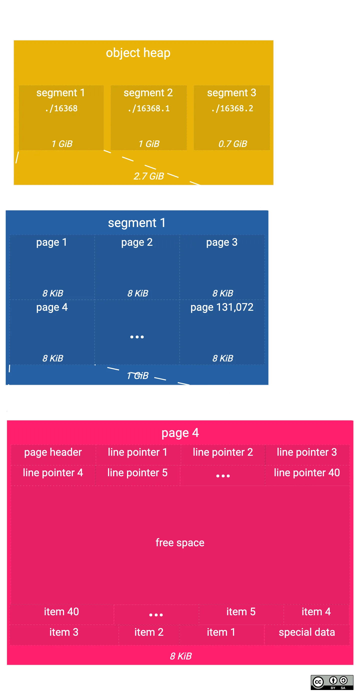
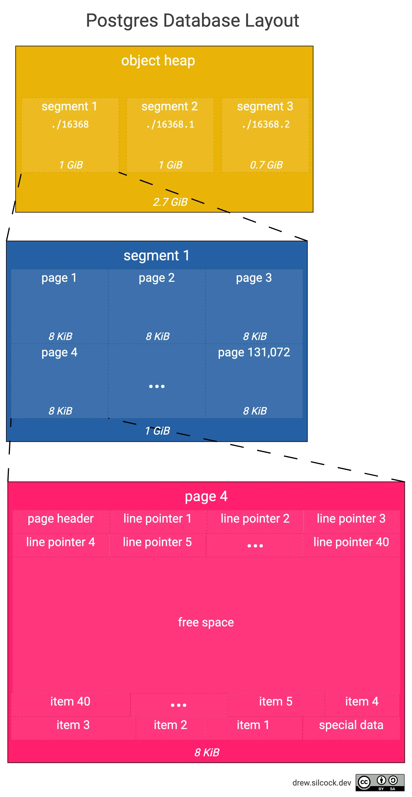
In our example here, our main table is 2.7 GiB which requires 3 separate segments of 1 GiB each. 131,072 pages of size 8 KiB into 1 GiB and each page consists of around 40 items (based on each item taking up about 200 bytes).
Page layout
Let’s dive down into our page layout.
You can see that there are three areas of the page:
- The header & line pointers, which grow “upwards”, meaning line pointer n + 1 has a higher initial offset into the page than line pointer n – the end of the final line pointer is called “lower”.
- The special data & items which grow “downwards”, meaning item n + 1 has a lower initial offset into the page than item n – the end of the final item is called “upper”.
- The free space, which is in between the last line pointer and the last item, i.e. goes from “lower” to “upper” – you can calculate the remaining free space in the page by doing “upper” - “lower”.
The page header itself contains things like:
- A checksum of the page
- The offset to the end of the line pointers (a.k.a. “lower”)
- The offset to the end of the free space (i.e. to the start of the items, a.k.a. “upper”)
- The offset to the start of the special space
- Version information
There’s actually an in-built extension called pageinspect which we can use to look at our page header information:
1blogdb=# create extension pageinspect;2CREATE EXTENSION3
4blogdb=# select * from page_header(get_raw_page('countries', 0));5    lsn    | checksum | flags | lower | upper | special | pagesize | version | prune_xid6-----------+----------+-------+-------+-------+---------+----------+---------+-----------7 0/1983F70 |        0 |     0 |   292 |   376 |    8192 |     8192 |       4 |         08(1 row)9
10blogdb=# select * from page_header(get_raw_page('countries', 1));11    lsn    | checksum | flags | lower | upper | special | pagesize | version | prune_xid12-----------+----------+-------+-------+-------+---------+----------+---------+-----------13 0/19858E0 |        0 |     0 |   308 |   408 |    8192 |     8192 |       4 |         014(1 row)15
16blogdb=# select * from page_header(get_raw_page('countries', 2));17    lsn    | checksum | flags | lower | upper | special | pagesize | version | prune_xid18-----------+----------+-------+-------+-------+---------+----------+---------+-----------19 0/1987278 |        0 |     0 |   296 |   416 |    8192 |     8192 |       4 |         020(1 row)21
22blogdb=# select * from page_header(get_raw_page('countries', 3));23    lsn    | checksum | flags | lower | upper | special | pagesize | version | prune_xid24-----------+----------+-------+-------+-------+---------+----------+---------+-----------25 0/19882C8 |        0 |     0 |   196 |  3288 |    8192 |     8192 |       4 |         026(1 row)
The first thing you might notice is that special is the same as pagesize – this is just saying that there is no special data section for this page. The special data section is not used for table pages, only for other types like indexes where it stores information about the binary tree structure.
You might be wondering why all the checksum values are all 0. Turns out that Postgres disables checksum protection by default for performance reasons and you have to manually enable it.
If we compare the lower and upper values for these pages, we can see that:
- Page 0 has 376 - 292 = 84 bytes of free space
- Page 1 has 408 - 308 = 100 bytes of free space
- Page 2 has 416 - 296 = 120 bytes of free space
- Page 3 has 3288 - 196 = 3092 bytes of free space.
We can infer from this that:
- The rows in our countries table is ~100 bytes as that’s how much space is left in the full pages.
- Page 3 is the final page as there’s plenty of space left in there.
We can confirm the row size using the heap_page_items() function from pageinspect:
1blogdb=# select lp, lp_off, lp_len, t_ctid, t_data2blogdb-# from heap_page_items(get_raw_page('countries', 1))3blogdb-# limit 10;4 lp | lp_off | lp_len | t_ctid | t_data5----+--------+--------+--------+------------------------------------------------------------------------------------------------------------------------------------------------------------------------------------------------------------------------------------------------------------6 1 | 8064 | 123 | (1,1) | \x440000002545717561746f7269616c204775696e656107475109474e51093232361d49534f20333136362d323a47510f416672696361275375622d5361686172616e204166726963611d4d6964646c65204166726963610930303209323032093031377 2 | 7944 | 114 | (1,2) | \x45000000114572697472656107455209455249093233321d49534f20333136362d323a45520f416672696361275375622d5361686172616e204166726963611f4561737465726e204166726963610930303209323032093031348 3 | 7840 | 97 | (1,3) | \x46000000114573746f6e696107454509455354093233331d49534f20333136362d323a45450f4575726f7065214e6f72746865726e204575726f7065030931353009313534092020209 4 | 7720 | 116 | (1,4) | \x47000000134573776174696e6907535a0953575a093734381d49534f20333136362d323a535a0f416672696361275375622d5361686172616e2041667269636121536f75746865726e2041667269636109303032093230320930313810 5 | 7600 | 115 | (1,5) | \x4800000013457468696f70696107455409455448093233311d49534f20333136362d323a45540f416672696361275375622d5361686172616e204166726963611f4561737465726e2041667269636109303032093230320930313411 6 | 7448 | 148 | (1,6) | \x490000003946616c6b6c616e642049736c616e647320284d616c76696e61732907464b09464c4b093233381d49534f20333136362d323a464b13416d657269636173414c6174696e20416d657269636120616e64207468652043617269626265616e1d536f75746820416d657269636109303139093431390930303512 7 | 7344 | 103 | (1,7) | \x4a0000001d4661726f652049736c616e647307464f0946524f093233341d49534f20333136362d323a464f0f4575726f7065214e6f72746865726e204575726f70650309313530093135340920202013 8 | 7248 | 89 | (1,8) | \x4b0000000b46696a6907464a09464a49093234321d49534f20333136362d323a464a114f6365616e6961154d656c616e657369610309303039093035340920202014 9 | 7144 | 97 | (1,9) | \x4c0000001146696e6c616e640746490946494e093234361d49534f20333136362d323a46490f4575726f7065214e6f72746865726e204575726f70650309313530093135340920202015 10 | 7048 | 95 | (1,10) | \x4d0000000f4672616e636507465209465241093235301d49534f20333136362d323a46520f4575726f70651f5765737465726e204575726f70650309313530093135350920202016(10 rows)Here lp means the line pointer, lp_off means the offset to the start of the item, lp_len is the size of the item in bytes and t_ctid refers to the ctid of the item. The ctid (Current Tuple ID)5 tells you where the item is located in the form (page index, item index within page) so (1, 1) means the first item in page 1 (pages are zero-indexed, item index is not for some reason).
We can also see the actual data for the item here as well, which is pretty cool – this long hex string is exactly the bytes that Postgres has stored on disk. Let’s check which row we’re looking at with some Python:
1$ row_data=$(docker exec $pg_container_id psql -U postgres blogdb --tuples-only -c "select t_data from heap_page_items(get_raw_page('countries', 1)) limit 1;")2# You can replace `hexyl` with `xxd` if you don't have hexyl installed.3$ echo "$row_data" | cut -c4- | xxd -r -p | hexyl4$ hexyl row_data.bin5┌────────┬─────────────────────────┬─────────────────────────┬────────┬────────┐6│00000000│ 44 00 00 00 25 45 71 75 ┊ 61 74 6f 72 69 61 6c 20 │D⋄⋄⋄%Equ┊atorial │7│00000010│ 47 75 69 6e 65 61 07 47 ┊ 51 09 47 4e 51 09 32 32 │Guinea•G┊Q_GNQ_22│8│00000020│ 36 1d 49 53 4f 20 33 31 ┊ 36 36 2d 32 3a 47 51 0f │6•ISO 31┊66-2:GQ•│9│00000030│ 41 66 72 69 63 61 27 53 ┊ 75 62 2d 53 61 68 61 72 │Africa'S┊ub-Sahar│10│00000040│ 61 6e 20 41 66 72 69 63 ┊ 61 1d 4d 69 64 64 6c 65 │an Afric┊a•Middle│11│00000050│ 20 41 66 72 69 63 61 09 ┊ 30 30 32 09 32 30 32 09 │ Africa_┊002_202_│12│00000060│ 30 31 37 0a ┊ │017_ ┊ │13└────────┴─────────────────────────┴─────────────────────────┴────────┴────────┘14$ docker exec $pg_container_id psql -U postgres blogdb -c "select * from countries where name = 'Equatorial Guinea';"15 ctid | id | name | alpha_2 | alpha_3 | numeric_3 | iso_3166_2 | region | sub_region | intermediate_region | region_code | sub_region_code | intermediate_region_code16-------+----+-------------------+---------+---------+-----------+---------------+--------+--------------------+---------------------+-------------+-----------------+--------------------------17 (1,1) | 68 | Equatorial Guinea | GQ | GNQ | 226 | ISO 3166-2:GQ | Africa | Sub-Saharan Africa | Middle Africa | 002 | 202 | 01718(1 row)Ahah, we are looking at the data for Equatorial Guinea, the only continental African country to speak Spanish as an official language. (If you’re wondering why (1,1) isn’t Afghanistan, the country with ID 1, remember that the pages start at 0 so we’d expect to find Afghanistan at (0,1).)
We can see here that each column is being stored right next to each other with a random byte in between each one. Let’s dive in:
0x 44 00 00 00=68(must be little endian) so the first 4 bytes is the row’s ID- Then, there’s a random byte like
0x25or0x07followed by the column data – the rest of the columns are string types so they’re all stored in UTF-8. If you know what these inter-column bytes mean, leave a comment below! I can’t figure it out. Edit: Thanks for everyone who commented with their insight on this. For an in-depth explanation, see the part 2 follow-on post: How Postgres stores oversized values – let’s raise a TOAST.
Individual values that are too big to store in here (e.g. they’re more than 8 KiB in size) get stored in a separate relation, or TOASTed – this will be the topic of a future post 🍞.
What happens when a row gets modifed or deleted?
Postgres uses MVCC (Multiversion Concurrency Control) to handle concurrent access to data. The “multiversion” here means that when a transaction comes in and modifies a row, it doesn’t touch the existing tuple on disk at all. Instead, it creates a new tuples at the end of the last page with the modified row. When it commits the update, it swaps the version of the data that a new transaction will see from the old tuple to the new one.
Let’s see this in action:
1blogdb=# select ctid from countries where name = 'Antarctica';2 ctid3-------4 (0,9)5(1 row)6
7blogdb=# update countries set region = 'The South Pole' where name = 'Antarctica';8UPDATE 19
10blogdb=# select ctid from countries where name = 'Antarctica';11  ctid12--------13 (3,44)14(1 row)15
16blogdb=# select lp, lp_off, lp_len, t_ctid, t_data17blogdb-# from heap_page_items(get_raw_page('countries', 0))18blogdb-# offset 8 limit 1;19 lp | lp_off | lp_len | t_ctid | t_data20----+--------+--------+--------+--------21  9 |      0 |      0 |        |22(1 row)
We can see that once we update the row, its ctid changes from (0,9) to (3,44) (which is probably at the end of the last page). The old data and ctid is also wiped from the old item location.
What about deletions? Let’s take a look:
1blogdb=# delete from countries where name = 'Equatorial Guinea';2DELETE 13
4blogdb=# select lp, lp_off, lp_len, t_ctid, t_data5blogdb-# from heap_page_items(get_raw_page('countries', 1))6blogdb-# limit 1;7 lp | lp_off | lp_len | t_ctid |                                                                                                  t_data8----+--------+--------+--------+----------------------------------------------------------------------------------------------------------------------------------------------------------------------------------------------------------9  1 |   8064 |    123 | (1,1)  | \x440000002545717561746f7269616c204775696e656107475109474e51093232361d49534f20333136362d323a47510f416672696361275375622d5361686172616e204166726963611d4d6964646c652041667269636109303032093230320930313710(1 row)
The data is still there! That’s because Postgres doesn’t bother actually deleting the data, it just marks the data as deleted. But you might be thinking, if rows are constantly getting deleted and added, you’ll end up with constantly increasing segments files full of deleted data (called “dead tuples” in the Postgres lingo). This is where vacuuming comes in. Let’s trigger a manual vacuum and see what happens.
1blogdb=# vacuum full;2VACUUM3
4blogdb=# select lp, lp_off, lp_len, t_ctid, t_data5blogdb-# from heap_page_items(get_raw_page('countries', 1))6blogdb-# limit 1; -- This used to be the dead tuple where 'Equatorial Guinea' was.7 lp | lp_off | lp_len | t_ctid |                                                                        t_data8----+--------+--------+--------+------------------------------------------------------------------------------------------------------------------------------------------------------9  1 |   8088 |     97 | (1,1)  | \x46000000114573746f6e696107454509455354093233331d49534f20333136362d323a45450f4575726f7065214e6f72746865726e204575726f70650309313530093135340920202010(1 row)11
12blogdb=# select lp, lp_off, lp_len, t_ctid, t_data13blogdb-# from heap_page_items(get_raw_page('countries', 0))14blogdb-# offset 8 limit 1; -- This used to be the dead tuple where the old 'Antarctica' version was.15 lp | lp_off | lp_len | t_ctid |                                                                                                               t_data16----+--------+--------+--------+------------------------------------------------------------------------------------------------------------------------------------------------------------------------------------------------------------------------------------17  9 |   7192 |    136 | (0,9)  | \x0a00000029416e746967756120616e64204261726275646107414709415447093032381d49534f20333136362d323a414713416d657269636173414c6174696e20416d657269636120616e64207468652043617269626265616e1543617269626265616e09303139093431390930323918(1 row)19
20blogdb=# select ctid, name from countries21blogdb-# where name = 'Antarctica' or ctid = '(0,9)' or ctid = '(1,1)';22  ctid  |        name23--------+---------------------24 (0,9)  | Antigua and Barbuda25 (1,1)  | Estonia26 (3,42) | Antarctica27(3 rows)
Now that we’ve vacuumed, a couple of things have happened:
- The dead tuple where the outdated first version of the Antarctica row was located has now been replaced with Antigua and Barbuda, which is the next country along.
- The dead tuple where the Equatorial Guinea row was located has now been replaced with Estonia, the next country along.
- Antarctica has moved from
(3,44)down to(3,42)because the 2 dead tuples has now been cleaned out and the Antarctica row can move down 2 slots.
What about indexes?
Indexes work exactly the same as tables! The only difference is that the tuple stored as items in each page contains the indexed data instead of the full row data and the special data contains sibling node information for the binary tree.
Exercise for the reader: Find the segment file for the name column unique index and investigate the values of the t_data in each item and “special data” for each page. Comment below what you find!
Why would I ever need to know any of this?
There’s a few reasons:
- It’s interesting!
- It helps understand how Postgres queries your data on disk, how MVCC works and lots more that’s really useful when you’re trying to gain a deep understanding of how your database works for the purpose of fine-tuning performance.
- In certain rare circumstances, it can actually be quite useful for data recovery. Take the following examples:
- You have someone who through incompetence or malice decides to corrupt your database by removing or messing up a couple of files on disk. Postgres can no longer understand the database so starting Postgres up will just result in a corrupted state. You can swoop in and use your knowledge to manually recover the data. This would still be a fairly large undertaking to do this, and in real life you’d probably call in a professional data recovery specialist, but maybe in this imaginary scenario your company can’t afford one so you have to make do.
- Someone accidentally set the super-important customers table on the production database as unlogged6 and then the server crashes. Because in an unlogged table changes aren’t written to the WAL, a database recovery via logical decoding will not include any of the unlogged table data. If you restart the server, Postgres will wipe clean the whole unlogged table because it will restore the database state from the WAL. However, if you copy out the raw database files, you can use the knowledge you have gained from this post to recover the contents of the data. (There’s probably a tool that does this already, but if not you could write your own – that would be an interesting project…)
- It’s a good conversation starter at parties 7.
Further reading
- Ketan Singh – How Postgres Stores Rows
- PostgreSQL Documentation – Chapter 73. Database Physical Storage
- Advanced SQL (Summer 2020), U Tübingen – DB2 — Chapter 03 — Video #09 — Row storage in PostgreSQL, heap file page layout
- 15-445/645 Intro to Database Systems (Fall 2019), Carnegie Mellon University – 03 - Database Storage I
- Structure of Heap Table in PostgreSQL
- pgPedia – Data Directory
Future topics
Database engines is an endlessly interesting topic, and there’s lots more I’d like to write about in this series. Some ideas are:
- How Postgres stores oversized values – let’s raise a TOAST
- How Postgres handles concurrency – MVCC is the real MVP
- How Postgres turns a SQL string into data
- How Postgres ensures data integrity – where’s WAL
If you’d like me to write about one of these, leave a comment below 🙂
Updates
- 2024-08-05: Rephrased the explanation of logical decoding based on HN comment from dfox, added explanation of why checksums are all 0 after HN discussion, expanded teaser for future TOAST post.
- 2024-08-15: On suggestion of jmholla on HN, replace Python decoding with xxd tool one-liner.
Footnotes
-
Technically, the data directory is whatever you specify in environment variable
PGDATAand it’s possible to put some of the cluster config files elsewhere, but the only reason you’d be messing with any of that is if you were hosting multiple clusters on the same machine using different Postgres server instances, which is a more advanced use case than we’re interesting in here. ↩ -
You might be wondering why the numeric country code is stored as
char(3)instead ofinteger. You could store it as an integer if you want, but – exactly like phone numbers – it doesn’t make any sense to say “Austria ÷ Afghanistan = Antarctica” (even though numerically it’s true) so what’s the point in storing it as an integer? Really it’s still a 3-character identifier, it’s just restricting the available characters to 0-9 instead of a-z as with the alpha-2 and alpha-3 country codes. ↩ -
The relfilenode may start off equal to oid as we can see here but it will change over time, e.g. after a
vacuum fullortruncate. ↩ -
There’s also a filed called
{filenode}_initwhich is used to store initialisation information for unlogged tables, but you won’t see these unless you’re using unlogged tables. ↩ -
I think this is what the C stands for but I’m not sure. ↩
-
You can pretend that you’ve never accidentally run a query on prod instead of your local dev database, but we all do it sooner or later. ↩
-
It’s not, please don’t do this unless you don’t want to be invited back to said parties. ↩